Next: Description, Up: (dir) [Contents]
This manual is for Cplint R program version 1.0.0
| • Description: | A brief description of what this is all about | |
| • Installation: | Installation procedures on various systems | |
| • Examples: | Trivial examples to explain how to use the library | |
| • Protocol: | Formal descriprion of the protocol | |
| • Development: | A thorough description on how to develop this library | |
| • Thanks: | People and communities | |
| • References: | References to the technologies used |
Next: Installation, Previous: Top, Up: Top [Contents]
The purpose of this library is to provide an interface between the Cplint1 suite for SWI Prolog2 and R3 to handle charts made with the ggplot24 package.
This means that most C3js5 charting functions of Cplint are also available for R.
In order to simplify the understanding of this document, a minimal set of terminology is necessary:
< > represents pseudocode.
# represents an unsigned integer or the root user,
depending on the context.
[ ].
Next: Examples, Previous: Description, Up: Top [Contents]
Cplint R is provided as part of the Cplint on SWISH6 package. This is the recomended and simplest way to obtain a working installation without too much trouble.
You can also install it manually with pack_install('cplint_r').
using the swipl command on UNIX-like systems. Unfortunately, doing
this is not enough since you need to setup an R environment with the
components described in the following section. For more information, have a
look at the
SWISH Installer Manual7
Cplint R has both Prolog and R dependencies:
Next: Protocol, Previous: Installation, Up: Top [Contents]
The following is the content of gauss_mean_est_R.pl.
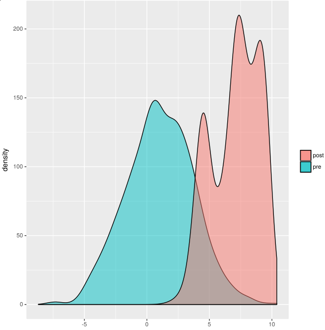
/*
Posterior estimation in Bayesian models.
We are trying to estimate the true value of a Gaussian distributed random
variable, given some observed data. The variance is known (2) and we
suppose that the mean has a Gaussian distribution with mean 1 and variance
5. We take different measurement (e.g. at different times), indexed
with an integer.
Given that we observe 9 and 8 at indexes 1 and 2, how does the distribution
of the random variable (value at index 0) changes with respect to the case of
no observations?
From
http://www.robots.ox.ac.uk/~fwood/anglican/examples/viewer/?worksheet=gaussian-posteriors
*/
:- use_module(library(mcintyre)).
:- use_module(library(cplint_r)).

:- mc.
:- begin_lpad.

value(I,X) :-
  mean(M),
  value(I,M,X).
% at time I we see X sampled from a Gaussian with mean M and variamce 2.0

mean(M): gaussian(M,1.0, 5.0).
% Gaussian distribution of the mean of the Gaussian of the variable

value(_,M,X): gaussian(X,M, 2.0).
% Gaussian distribution of the variable


:- end_lpad.

hist_uncond(Samples,NBins):-
  mc_sample_arg(value(0,X),Samples,X,L0),
  histogram_r(L0,NBins).
% plot an histogram of the density of the random variable before any
% observations by taking Samples samples and by dividing the domain
% in NBins bins

dens_lw(Samples):-
  mc_sample_arg(value(0,Y),Samples,Y,L0),
  mc_lw_sample_arg(value(0,X),(value(1,9),value(2,8)),Samples,X,L),
  densities_r(L0,L).
% plot the densities of the random variable before and after
% observing 9 and 8 by taking Samples samples.


/** <examples>
?- dens_lw(1000).
% plot the densities of the random variable before and after
% observing 9 and 8
?- hist_uncond(10000,40).
% plot an histogram of the density of the random variable before any
% observations
?-  mc_lw_expectation(value(0,X),(value(1,9),value(2,8)),1000,X,E).
% E = 7.166960047178755
?- mc_expectation(value(0,X),10000,X,E).
% E = 0.9698875384639362.

*/
Using ?- dens_lw(1000) as query the following chart is produced:
For other examples see all the files ending in "_R.pl" on https://github.com/friguzzi/swish/tree/master/examples/inference
Next: Development, Previous: Examples, Up: Top [Contents]
The following is a list of exported predicates available to the library users’.
Each predicate corresponds to one of the following categories
Each argument of a predicate correponds to a data type. See the SWI Prolog data types manual12 and the Learn Prolog Now manual13. Have a look at the Cplint help manual14 to learn in details about the functionality of each predicate.
Given to lists X and Y build an output list Out
in the form [X1-Y1,X2-Y2,...,XN-YN].
Given two atoms X and Y, build the term r(X,Y)
in Out.
Given an input list L in the form [X1-Y1,X2-Y2,...,XN-YN],
transform it in an output list R in the form
[r(X1,Y1),r(X2,Y2),...,r(XN,YN)].
This means that R will contain an X-Y relationship
which can be then passed to an R data frame.
The predicate computes and plots the probability of Query as a bar chart with a bar for the probability of Query true and a bar for the probability of Query false. If Query is not ground, it returns in backtracking all ground instantiations of Query together with their probabilities.
The predicate computes and plots the probability of Query given Evidence as a bar chart with a bar for the probability of Query true and a bar for the probability of Query false given Evidence. If Query / Evidence are not ground, it returns in backtracking all ground instantiations of Query / Evidence together with their probabilities.
See prob_bar_r/2.
The predicate samples Query a number of Samples times and plots a bar chart with a bar for the number of successes and a bar for the number of failures. If Query is not ground, it considers it as an existential query.
The predicate samples Query Samples times. Arg should be a variable in Query. The predicate plots a bar chart with a bar for each possible value of L, the list of values of Arg for which Query succeeds in a world sampled at random. The size of the bar is the number of samples returning that list of values.
The predicate samples Query Samples times. Arg should be a variable in Query. The predicate plots a bar chart with a bar for each value of Arg returned as a first answer by Query in a world sampled at random. The size of the bar is the number of samples that returned that value. The value is failure if the query fails.
The predicate calls mc_rejection_sample_arg/5 and builds an R graph
of the results.
It plots a bar chart with a bar for each possible value of L,
the list of values of Arg for which Query succeeds
given that Evidence is true
The size of the bar is the number of samples
returning that list of values.
The predicate calls mc_mh_sample_arg/6 and builds an R graph
of the results.
The predicate plots a bar chart
with a bar for each possible value of L,
the list of values of Arg for which Query succeeds in
a world sampled at random.
The size of the bar is the number of samples
returning that list of values.
The predicate calls mc_mh_sample_arg/7 and builds an R graph
of the results.
The predicate plots a bar chart
with a bar for each possible value of L,
the list of values of Arg for which Query succeeds in
a world sampled at random.
The size of the bar is the number of samples
returning that list of values.
Draws a histogram of the samples in List dividing the domain in NBins bins. List must be a list of couples of the form [V]-W or V-W where V is a sampled value and W is its weight.
Display a smooth density estimate of a sets of samples. The samples are in List as couples V-W where V is a value and W its weigth.
Display a smooth density estimate of two sets of samples, usually prior and post observations. The samples from the prior are in PriorList while the samples from the posterior are in PostList as couples V-W where V is a value and W its weigth.
The predicate takes as input a list LG of pairs probability-literal in asceding order on probability where the literal can be an Atom (incading a positive example) or \+ Atom, indicating a negative example while the probability is the probability of Atom of being true. PR and ROC diagrams are plotted. The predicate returns:
See http://cplint.lamping.unife.it/example/exauc.pl for an example.
Important predicates in this library follow a common structure to avoid confusion and promote standardization.
Interface predicates are involved in the interaction between input data from a program and the plot of that same data. These predicates are usable from the programs.
As the name suggests, plotting predicates are only involved in plotting the data.
Finally there are other functions which handle the lists and other types of data.
All interface predicates have a similar structure. Their names
end with _r (except the Helpers) in order to distinguish them from the
original Cplint predicates.
First and last operations are always load_r_libraries and
finalize_r_graph respectively.
Plotting is done right before the last operation with one of the geom_
predicates.
A skeleton of the structure follows.
<cplint_graphing_predicate>_r(<input>):-
    load_r_libraries,
    <operations on the input>,
    geom_<something>(<new input, possibly lists>),
    finalize_r_graph.
Predicates directly involved in plotting all start with geom_ as prefix.
These predicates work with lists which are then transformed into R data frames, and, as a final instruction, a corresponding plot is generated.
You can visualize the structure with the following pseudocode:
geom_<something>(<Lists and/or other input>) :-
    <handle lists>,
    <create one or more R data frame with the lists data>,
    <rename data frame colnames to avoid using default ones>,
    <- ggplot <something>
List handling is useful to pass information between Prolog and
R. This is done thanks to build_xy_list/3, r_row/3
and get_set_from_xy_list/2 predicates,
described in the interface section.
In case there are multiple distributions we simply have to call
get_set_from_xy_list/2 the appropriate number of times,
like: get_set_from_xy_list(<something>,R#).
As descibed before, a data frame is useful to pass structured information between Prolog and R.
In Cplint R in particular, we use r_data_frame_from_rows/2 provided by
the Rserve Client library, in the following
manner:
r_data_frame_from_rows(df[#], R[#])
For each distribution the optional number is incremented by one.
In case it is the last (or only) data frame then its name
will simply be df.
What follows are extracts of some trivial predicates indicated as internal helpers.
bin_width(Min,Max,NBins,Width) :-
  D is Max-Min,
  Width is D/NBins.

load_r_libraries :-
    <- library("ggplot2").

finalize_r_graph :-
    r_download.
You are welcomed to change this library. In order to test it you simply have to place you modified version in the correct path and restart SWISH. If you have used the packages provided with SWISH Installer this can be achieved with the following:
# mv <your_modified_cplint_r_library> /home/swish/lib/swipl/pack/cplint_r/prolog/cplint_r.pl
# systemctl restart swish-cplint
The source of this documentation is under the doc directory of the repository.
To be able to compile it, you have to install several tex packages
(for example: texlive-most and texi2html if you are using
Arch Linux) that contain the following binaries:
makeinfo
texi2dvi
docbook2html
docbook2pdf
docbook2txt
texi2html
perl
After running make, a directory named manual
will be created and you can access all the files by opening
index.html with a browser.
Next: References, Previous: Development, Up: Top [Contents]
Fabrizio Riguzzi for developement, testing and feedback.
Raivo Laanemets for a blog article15 on how to write SWI Prolog packs.
Some quotations reported here are taken directly from the respective web sites.
See item [Cplint] in Cplint.
See item [SWI Prolog] in SWI Prolog.
See item [R] in R.
See item [ggplot2] in ggplot2.
See item [C3js] in C3js.
See item [Cplint on SWISH] in Cplint on SWISH.
See item [SWISH Installer Manual] in SWISH Installer Manual.
See item [Rserve Client] in Rserve Client.
See item [R SWISH] in R SWISH.
See item [Rserve] in Rserve.
See item [gridExtra] in gridExtra.
See item [SWI Prolog data types] in SWI Prolog data types.
See item [LPN] in LPN.
See item [Cplint] in Cplint.
See item [Prolog pack development experience] in Prolog pack development experience.